The linear method of calculating depreciation of fixed assets - the essence of the technique
When choosing the linear method, depreciation is accrued every month for each fixed asset separately, depending on its useful life (clause 2 of Article 259 of the Tax Code of the Russian Federation).
The straight-line depreciation method implies that the following formula for calculating depreciation charges is used:
Am = OS × k
Where
Am – the amount of depreciation charges for the month;
k – monthly depreciation rate, expressed as a percentage;
OS is the initial or replacement cost of a depreciable fixed asset.
The depreciation rate for each fixed asset item is determined based on its useful life in months and is calculated using the formula:
k = (1/n) × 100%
where n is the number of months of useful use of the fixed asset.
This indicator is established on the basis of the Classification of fixed assets included in depreciation groups, approved by Decree of the Government of the Russian Federation dated January 1, 2002 No. 1 (hereinafter referred to as the Classification of fixed assets).
ATTENTION! The amount of depreciation calculated using the linear method is the same in accounting and tax accounting. Except in cases where bonus depreciation is applied.
ConsultantPlus experts explained how to calculate depreciation in tax accounting. Get trial access and upgrade to the Ready Solution for free.
Uniform attribution to expenses of the cost of depreciable fixed assets is the main convenience of the linear method.
of the enterprise in question
Home Favorites Random article Educational New additions Feedback FAQ⇐ PreviousPage 5 of 9Next ⇒
| Index | Recommended rate | At the beginning of the reporting period | At the end of the reporting period | Deviation |
| Debt to equity ratio | £ 1 | 0,862 | 1,159 | +0,297 |
| Long-term leverage ratio | £ 1 | — | — | — |
| Own funds maneuverability coefficient | 0,2-0,5 | 0,609 | 0,647 | +0,038 |
| Depreciation accumulation rate | 0,35 | 0,701 | 0,742 | +0,041 |
| Coefficient of real value of fixed assets in the property of the enterprise | ³ 0,5 | 0,210 | 0,163 | -0,047 |
| The coefficient of the real value of fixed assets and material current assets in the property of the enterprise | ³ 0,5 | 0,319 | 0,257 | -0,062 |
The ratio of borrowed (raised) and equity funds is the quotient of dividing the total amount of liabilities for borrowed (raised) funds (credits, borrowings, accounts payable) Сз to the amount of equity (equity) Сс, i.e. the sum of the indicators of lines 590 and 690 of the balance sheet, divided by the indicator of line 490. The ratio of borrowed and equity funds shows how much borrowed funds the company attracted per 1 ruble. own funds invested in assets. For the analyzed enterprise at the beginning of the year K
с = (1081711/1254705) = 0.862, at the end of the year
K
с = (1435579/1238485) = 1.159.
This is the most important indicator characterizing the financial autonomy (independence) of an enterprise. In the example under consideration, the financial independence of the enterprise remained very low: at the beginning of the year, by 1 rub. own funds accounted for 86.2 kopecks. borrowed, by the end of the year by 1 rub. own funds accounted for 1,159 rubles. borrowed, which is significantly higher than the criterion value.
With an increase in the ratio of borrowed and equity funds, the enterprise's dependence on borrowed funds increases and it gradually loses its financial stability.
The financial autonomy and stability of the enterprise is considered ensured when K
c < 0.7.
It is often believed that when K
c > 1, the financial position of the enterprise becomes critical.
However, this is not always the case. At high working capital turnover rates, the critical value of Kc
can far exceed one without significant consequences for the financial autonomy of the enterprise.
The long-term borrowing ratio is calculated as the ratio of the amount of long-term loans and borrowings to the amount of own CC and long-term borrowed funds, i.e. the quotient of dividing the indicator of line 590 of the balance sheet by the sum of lines 490 and 590. The long-term borrowing ratio indicates the share of long-term loans raised to finance the assets of the enterprise along with its own funds. The enterprise in question did not resort to long-term borrowings (credits and borrowings) during the year.
The coefficient of maneuverability of own funds (equity capital) is the quotient of the division of own working capital Co by the total amount of sources of own funds (equity capital): K
m = Co/Cs, i.e.
the difference between the indicators of lines 490 and 190, related to the indicator of line 490. The agility coefficient shows the degree of mobility (flexibility) in the use of own funds. According to Table 10, it can be seen that this indicator for the organization at the beginning of the year was 0.609 (60.9%), and at the end of the year 0.647 (64.7%). This means that the organization is provided with its own working capital and by the end of the year the supply increased by 3.8%. If K
m < 0, the organization lacks its own working capital.
The coefficient of maneuverability of own funds was quite high and increased by the end of the year, which allows us to judge the strengthening of the financial autonomy of the enterprise. The upward trend of this indicator indicates an improvement in financial autonomy in the future.
The agility coefficient evaluates the ability of an enterprise to maintain the level of its own working capital and replenish working capital, if necessary, from its own sources. The recommended coefficient value is 0.2-0.5. The closer the indicator value is to the upper recommended limit, the more opportunities for financial maneuver the enterprise has.
In the literature, this indicator is also called the equity ratio, which is defined as the ratio of own working capital to the total working capital of the enterprise. The lower limit of the coefficient values is 0.1, the upper limit is 0.5.
The depreciation accumulation coefficient is the ratio of the amount of accumulated depreciation (wear and tear) for fixed assets Io.s and intangible assets In.a to the original cost of the depreciable property:
K
u = (Io.s + In.a)/( ),
where is the initial cost of fixed assets and intangible assets.
The depreciation accumulation coefficient characterizes the intensity of the release of immobilized (in fixed assets and intangible assets) funds.
According to the enterprise balance sheet at the beginning of the year K
and = 4638871/15434248 = 0.701, at the end of the year
K
and = 4557001/11073677 = 0.742.
The depreciation accumulation coefficient indicates that at the beginning of the reporting period more than 70% of the original cost of fixed assets was repaid by depreciation charges. An increase in this indicator by the end of the reporting period indicates an increase in the depreciation of fixed assets during the year. To estimate the rate of depreciation accumulation, the average depreciation rate is calculated, i.e. the ratio of the amount of depreciation charges for the reporting period to the initial (average annual) cost of fixed assets and intangible assets.
The initial cost of fixed assets by the end of the year decreased by 4,360,571 rubles. or by 28.3%. A decrease in the depreciation accumulation rate means that the company is renewing its fixed assets. In this case, the initial cost of fixed assets at the enterprise should increase by the end of the year.
The coefficient of the real value of fixed assets in the property of the enterprise is equal to the ratio of the residual value of fixed assets to the value of the property of the enterprise C, i.e. the quotient of dividing the balance line data 120 by the data line 300. The coefficient indicates how effectively the enterprise's funds are used for business activities. In the example under consideration = 489551/2336416 = 0.21 or 21.0% at the beginning of the year and = 436379/2674064 = 0.163 or 16.3% at the end of the year, which once again confirms a significant reduction in the enterprise’s fixed assets during the year.
The relative value of the real value of fixed assets at the enterprise at the beginning of the year was unacceptably low (21.0%), and by the end of the reporting period it was only 16.3%. With normal financial stability of the enterprise, this indicator should exceed 0.5.
The coefficient is a special case of the more general coefficient of the real value of fixed assets and material current assets in the property of an enterprise.
⇐ Previous5Next ⇒
Calculation of depreciation using the straight-line method - example
Let us explain with a specific example how the linear depreciation method is used in practice.
On March 18, 2020, a woodworking machine for furniture production was purchased from Gamma LLC and registered as a fixed asset at an initial cost of RUB 180,000.00. The useful life of the machine was set at 72 months, because This fixed asset belongs to the 4th depreciation group according to the Classification of fixed assets.
IMPORTANT! The value of assets classified as fixed assets in tax accounting is equal to 100 thousand rubles, and in accounting accounting - 40 thousand rubles. Read about the differences between accounting and tax accounting in the material “What applies to fixed assets of an enterprise.”
Let's calculate the amount of depreciation for one month:
Am = 180,000.00 x (1/72 × 100%) = RUB 2,500.00.
Since, with a linear month, depreciation starts from the month following the month the purchased machine was accepted onto the balance sheet, then starting from 04/01/2020, for 6 years (72 months), Gamma LLC will monthly expense a depreciation amount of 2 RUB 500.00
If you have access to ConsultantPlus, check whether you have correctly calculated and reflected depreciation in your accounting. If you don't have access, get a free trial of online legal access.
Shelf life indicator
The serviceability coefficient of fixed assets is an indicator opposite to the depreciation indicator. It is calculated as the ratio of the original (replacement) cost to the collected amount of depreciation (depreciation). The resulting total can also be multiplied by 100%. This indicator shows the share of unworn fixed assets. The indicator is calculated at the beginning and end of the reporting year. The fitness indicator can be calculated by subtracting from one or 100% the value of the wear indicator. If you sum up the wear and serviceability indicators, you get a total of 1 or 100%. Let's say the wear rate is 0.3 or 30%, respectively, the serviceability rate will be 0.7 or 70%. The serviceability indicator must exceed the wear rate and, as a percentage, be more than half of the total cost of fixed assets. The enterprise must control the degree of deterioration and serviceability of its fixed assets, update and modernize them in a timely manner. Fixed assets in good condition are the key to an uninterrupted production process, reducing the cost of finished products and increasing the company’s revenue.
Transition from non-linear to linear depreciation method
If a non-linear depreciation method was initially used, and later it was decided to use a linear one (the Tax Code allows changing depreciation methods, but not more than once every 5 years), then accountants may have a lot of questions in connection with such a transition.
- What useful life is used in the calculation? When switching to the straight-line depreciation method, deductions are calculated based on the remaining useful life of the asset. This period must be determined on the 1st day of the month of the tax period, when the use of the linear method begins (paragraph 2, paragraph 4, article 322 of the Tax Code of the Russian Federation).
- What value of the object should be taken as the basis for the new method of calculating depreciation? When switching to the linear depreciation method, you need to remember that part of the cost of the fixed asset has already been depreciated, so the calculation uses the residual value, which is also determined at the beginning of the tax period (clause 4 of Article 322 of the Tax Code of the Russian Federation). This is the position of officials (letter of the Federal Tax Service of Russia for Moscow dated December 1, 2009 No. 16-15/125942, letter of the Ministry of Finance of Russia dated January 28, 2010 No. 03-03-06/1/28).
- What should you do if, when switching to the straight-line depreciation method, the period of actual operation exceeded the useful life of the object, but the cost of the fixed asset was not completely written off as expenses? In such a situation, it is necessary to charge depreciation of the object until its value is written off (letter of the Ministry of Finance of Russia dated July 21, 2014 No. 03-03-RZ/35549). In this case, the useful life is determined by the taxpayer in accordance with the provisions of paragraph. 2 clause 7 art. 258 of the Tax Code of the Russian Federation and taking into account safety requirements and other factors affecting the wear and tear of the object.
How to work with property that has been used?
Organizations often operate objects that have already been used . Among them:
- Fixed assets received by an enterprise through succession when a legal entity was reorganized.
- Property received as a contribution to the authorized capital.
- Objects whose condition was not new already during the acquisition process
For such objects, depreciation is calculated in exactly the same way as for fixed assets. The only difference is that the service life is calculated slightly differently.
To determine it, we subtract from the period established by the former owners the time during which the equipment was actually used.
The main thing is to remember that the results of financial activities should not be affected by the absence or presence of these deductions at a particular enterprise. They are necessarily included in expenses for the tax period to which they relate.
It is acceptable to use non-linear methods of depreciation calculations, but it is the linear method that will be convenient, for example, for buildings or structures. And for other objects that are not directly used in production processes.
Methods for calculating depreciation of fixed assets:
Results
The straight-line method of calculating depreciation is used in both accounting and tax accounting. The calculated amount will be the same in both cases, except in cases where bonus depreciation is applied.
Sources:
- Tax Code of the Russian Federation
- Decree of the Government of the Russian Federation dated January 1, 2002 No. 1
You can find more complete information on the topic in ConsultantPlus. Free trial access to the system for 2 days.